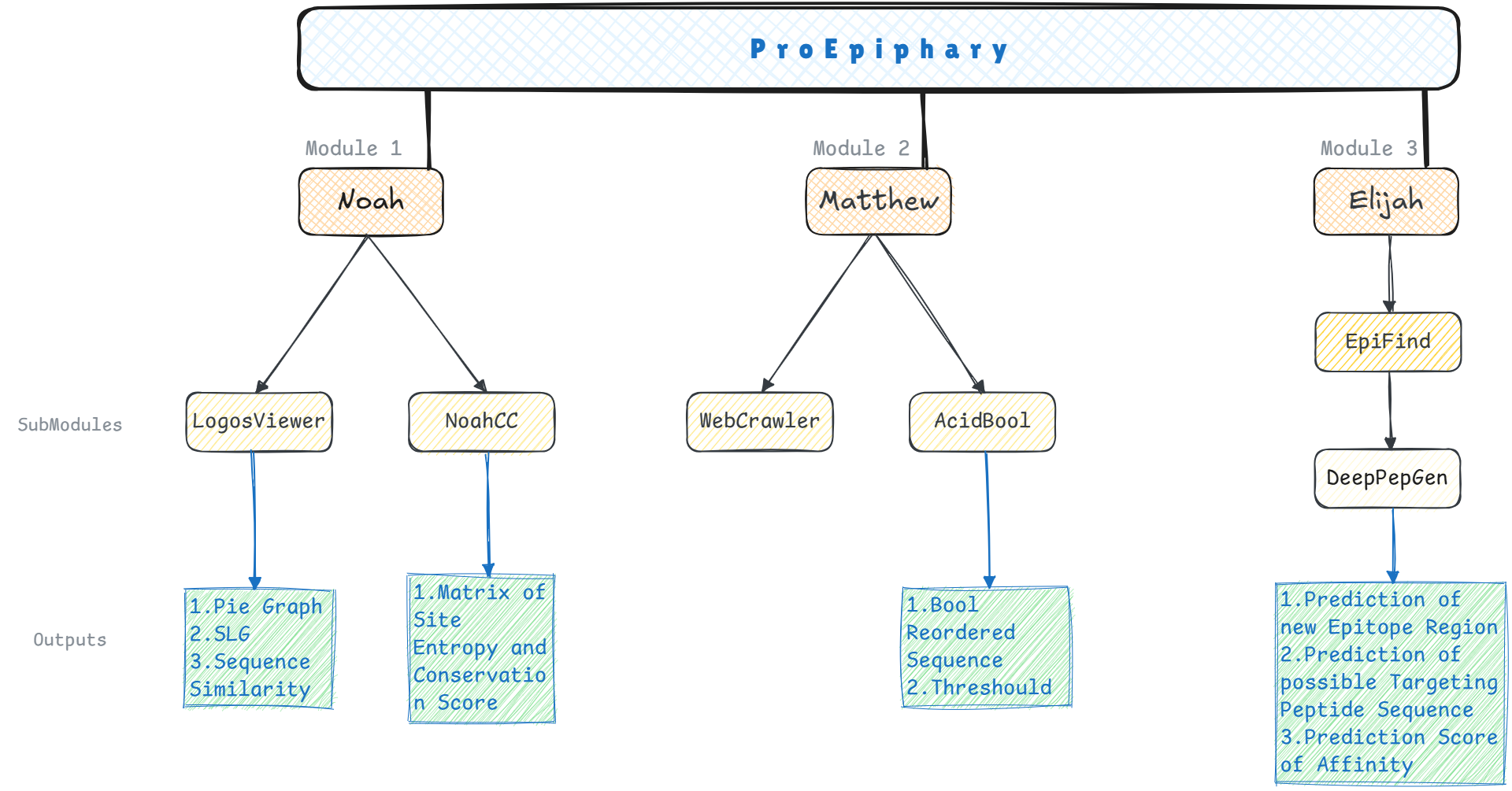
In protein-protein interaction (PPI)-based drug design, the intricate nature of microscopic structures often leads to inefficiencies and limited precision in wet-lab experiments. To address these challenges, we developed ProEpiphary, an integrated computational platform with AI technics that designed to enhance experimental efficiency and accuracy, mainly comprising three core modules (Fig.1):
Fig.1 | Framework of ProEpiphary.
Noah: This module integrates multi-scale computational biology algorithms to intelligently screen and score human AQP0 protein homologs, effectively assisting in sample selection and validation for wet-lab experiments.
Matthew: Utilizing data-driven sequence rearrangement models and some open-source tools, Matthew employs Machine Learning (ML) to analyze target-protein's surface properties, facilitating the design of targeted peptides.
Elijah: Incorporating the EpiFind and DeepPepGen submodules, Elijah, employing Deep Learning (DL) techniques such as Convolutional Neural Network (CNN), aims to characterize new epitopes automatically, generate target peptide sequence and predict the affinity of their combination. Meanwhile, the module also retains more room for future development. With sufficient experimental data and pretraining mechanisms, it is hoped to integrate with the two modules above, paving a full AI-driven workflow that accelerates drug discovery.
Modules
I. Noah
i. LogosViewer
In this module, we mainly employed a group of mathematical methods, named as Match Scoring Sequence Alignment Model (MSSAM):
S(i,j)1, S(i,j)2 denote the amino acid residues at position j in the i-th sequence pair
δ(x, y) is the Kronecker Delta Function:
\[\delta(x,y) = \begin{cases}
1 & \text{when } x = y \\
0 & \text{when } x \neq y
\end{cases} \quad \color{gray}{\textit{(Format.3)}}\]
3. Adjustment Factor (Analogous to HMM Transition Probability)
\[f = A^{(\frac{T-M}{T}\times k\times A)} + C \quad \color{gray}{\textit{(Format.4)}}\]
where:
A, B, C are Nonlinear Likelihood Correction Factor (NLCF), which can be implemented from the Convergence Process (CP) of parameters of the Hidden Markov Model (HMM). From articles [1][2] that analyzed these processes we have several methods that can solve the values of these parameters approximately, and results as Table.1 shows below:
\[S = (\frac{M}{T}) \times f \times 100 \quad \color{gray}{\textit{(Format.5)}}\]
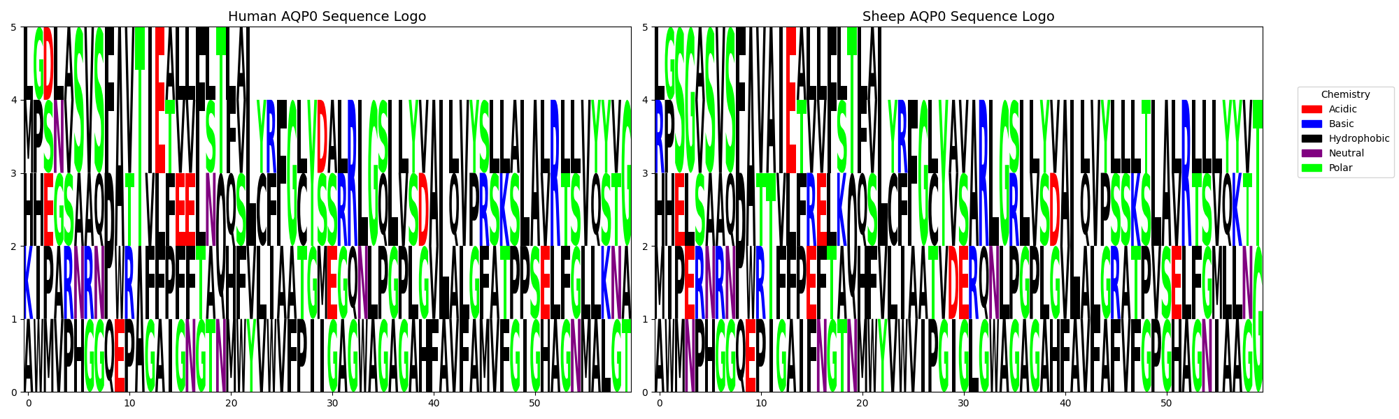
As excepted, LogosViewer conducts an amino acid composition analysis of two protein sequences, generates visual representations in form of Pie Charts (PC) (result shown in Fig.2) and sequence Logo Graph (SLG) (Fig.3), and computes the similarity (Code.1) between the two sequences.
Fig.2 | Comparison of amino acid frequency distribution between human and sheep AQP0.
Fig.3 | Sequence Logo Graph (SLG) visualization of the protein sequences.
Code.1 | Sequence similarity
Sequence similarity: 90.8292%
Code.2 | Source code of LogosViewer module
# Source Code (Code.2)
from collections import Counter
import matplotlib.pyplot as plt
import logomaker
import matplotlib.patches as mpatches
import os
import platform
import time
from datetime import datetime

print('''^^ProEpiphary^^ ''')
print('''Module: Noah-LogosViewer 3.5''')
print('''analyzing...''')

def read_sequences(file_path):
    """Read sequences from file"""
    with open(file_path, 'r') as file:
        sequences = file.readlines()
    sequences = [line.strip() for line in sequences if line.strip()]
    return sequences

def pad_sequences(sequences):
    """Pad sequences to equal length"""
    max_len = max(len(seq) for seq in sequences)
    padded_sequences = [seq.ljust(max_len, '-') for seq in sequences]
    return padded_sequences

def calculate_similarity(seq_list1, seq_list2):
    """Calculate similarity between two sequence lists"""
    if len(seq_list1) != len(seq_list2):
        raise ValueError("Sequence lists must have the same length for comparison.")

    total_positions = 0
    matching_positions = 0

    for seq1, seq2 in zip(seq_list1, seq_list2):
        if len(seq1) != len(seq2):
            raise ValueError("Each sequence pair must have the same length for comparison.")

        total_positions += len(seq1)
        matching_positions += sum(aa1 == aa2 for aa1, aa2 in zip(seq1, seq2))
        influrate = 0.99516105 ** ((total_positions - matching_positions) / total_positions * 99.516105) + 0.00483894

    similarity = (matching_positions / total_positions) * influrate * 100
    return similarity

def generate_combined_pie_chart(sequences1, sequences2, titles, file_name):
    """Generate pie charts for amino acid frequencies"""
    amino_acid_counts1 = Counter(''.join(sequences1).replace('-', ''))
    amino_acid_counts2 = Counter(''.join(sequences2).replace('-', ''))

    labels1, sizes1 = zip(*amino_acid_counts1.most_common())
    labels2, sizes2 = zip(*amino_acid_counts2.most_common())

    fig, axes = plt.subplots(1, 2, figsize=(14, 7))

    axes[0].pie(sizes1, labels=labels1, autopct='%1.1f%%', startangle=90)
    axes[0].set_title(titles[0], fontsize=14)
    axes[0].axis('equal')

    axes[1].pie(sizes2, labels=labels2, autopct='%1.1f%%', startangle=90)
    axes[1].set_title(titles[1], fontsize=14)
    axes[1].axis('equal')

    plt.tight_layout()
    plt.savefig(file_name)
    print(f"Pie chart saved: {file_name}")
    plt.close()

def generate_combined_logo(sequences1, sequences2, titles, file_name, custom_colors, legend_labels=None):
    """Generate sequence logo visualization"""
    fig, axes = plt.subplots(1, 2, figsize=(20, 6))

    logo_data1 = logomaker.alignment_to_matrix(sequences1, to_type='counts')
    logo_data2 = logomaker.alignment_to_matrix(sequences2, to_type='counts')

    logomaker.Logo(logo_data1, ax=axes[0], color_scheme=custom_colors)
    axes[0].set_title(titles[0], fontsize=14)

    logomaker.Logo(logo_data2, ax=axes[1], color_scheme=custom_colors)
    axes[1].set_title(titles[1], fontsize=14)

    if legend_labels:
        axes[1].legend(handles=legend_labels, loc='upper left', bbox_to_anchor=(1.05, 0.85), title='Chemistry')

    plt.tight_layout()
    plt.savefig(file_name)
    print(f"Sequence logo saved: {file_name}")
    plt.close()

# Color scheme for sequence logo
custom_colors = {
    letter: '#FF0000' for letter in 'DE'  # Acidic
}
custom_colors.update({
    letter: '#000000' for letter in 'ACFHIJLMOPQZWXUV'  # Hydrophobic
})
custom_colors.update({
    letter: '#0000FF' for letter in 'KR'  # Basic
})
custom_colors.update({
    letter: '#00FF00' for letter in 'TSGY'  # Polar
})
custom_colors.update({
    letter: '#800080' for letter in 'N'  # Neutral
})

legend_labels = [
    mpatches.Patch(color='#FF0000', label='Acidic'),
    mpatches.Patch(color='#0000FF', label='Basic'),
    mpatches.Patch(color='#000000', label='Hydrophobic'),
    mpatches.Patch(color='#800080', label='Neutral'),
    mpatches.Patch(color='#00FF00', label='Polar'),
]

if __name__ == "__main__":
    start_time = time.time()

    print("Enter the full path for human AQP0 sequence file (e.g., human aqp0.txt):")
    file1_path = input("Path 1: ").strip()
    print('Enter the full path for Sheep AQP0 sequence file (e.g., sheep aqp0.txt):')
    file2_path = input("Path 2: ").strip()
    print('''
    ''')

    if not os.path.exists(file1_path):
        print(f"Error: File not found -> {file1_path}")
        exit(1)
    if not os.path.exists(file2_path):
        print(f"Error: File not found -> {file2_path}")
        exit(1)

    sequences1 = read_sequences(file1_path)
    sequences2 = read_sequences(file2_path)

    if not sequences1 or not sequences2:
        print("One or both sequence files are empty.")
        exit(1)
    else:
        sequences1 = pad_sequences(sequences1)
        sequences2 = pad_sequences(sequences2)

        output_dir = os.path.dirname(file1_path)
        timestamp = datetime.now().strftime("%Y%m%d_%H%M%S")

        pie_chart_file = os.path.join(output_dir, f"Pie_Chart_( {timestamp} ).png")
        generate_combined_pie_chart(
            sequences1,
            sequences2,
            ["Human AQP0 Amino Acid Frequency", "Sheep AQP0 Amino Acid Frequency"],
            pie_chart_file
        )

        logo_file = os.path.join(output_dir, f"Sequence_Logo_( {timestamp} ).png")
        generate_combined_logo(
            sequences1,
            sequences2,
            ["Human AQP0 Sequence Logo", "Sheep AQP0 Sequence Logo"],
            logo_file,
            custom_colors,
            legend_labels
        )

        try:
            similarity = calculate_similarity(sequences1, sequences2)
            print(f"Sequence similarity: {similarity:.4f}%")
            print('''Mission completed, view the results in the source folder now...''')
        except ValueError as error:
            print(f"Error calculating similarity: {error}")

    end_time = time.time()
    runtime = end_time - start_time
    print("\n----- Local System Information -----")
    print(f"Processor: {platform.processor()}")
    print(f"Total runtime: {runtime:.2f} seconds")
    print('''v1.2   (Last Update:31/01/2025)''')
ii. NoahCC
NoahCC is designed to calculate Information Entropy (IE) values and Conservation Scores (CS) of specific sites of each sequence, enabling the quantitative analysis of biological conservation along with the identification of critical similarities and differences for further wet-lab experiments.
P(a,j) represents the relative frequency of amino acid a at position j
count(a,j) is the number of times a appears at position j
N is the total number of amino acids at that position
H(j) is the entropy of position j, lower H(j) values indicate higher conservation, meaning the position is more functionally or structurally important
C(j) is the conservation score of position j
max P(a,j) is the highest amino acid frequency at that position
ε is a small fixed adjustment factor to introduce a slight variability in the score [4]
Partial running result (values for the first 20 amino acids) is shown in Table.2 below. A lower IE value and a higher CS indicate that the site is relatively more conserved, which is crucial for its biological function and structure.
Table.2 | Partial running result (values for the first 20 amino acids)
Position
Human_Entropy
Human_ConScore
Sheep_Entropy
Sheep_ConScore
1
2.3219
0.55
2.3219
0.53
2
2.3219
0.54
2.3219
0.55
3
2.3219
0.55
1.9219
0.75
4
2.3219
0.59
1.9219
0.76
5
2.3219
0.57
2.3219
0.59
6
1.9219
0.78
1.9219
0.79
7
1.9219
0.76
1.9219
0.78
8
1.9219
0.76
1.9219
0.77
9
1.5219
0.76
1.5219
0.77
10
1.3710
0.92
1.3710
0.91
11
1.9219
0.76
1.9219
0.73
12
0.9710
0.91
1.5219
0.78
13
1.9219
0.72
1.9219
0.72
14
1.9219
0.79
1.9219
0.75
15
2.3219
0.56
2.3219
0.54
16
2.3219
0.52
2.3219
0.54
17
2.3219
0.56
2.3219
0.55
18
1.9219
0.76
1.9219
0.79
19
2.3219
0.55
2.3219
0.56
20
1.5219
0.72
1.5219
0.76
Source Code (Code.3) has been uploaded on GitHub, and can be viewed below:
Code.3 | Source code of NoahCC module
import numpy as np
from collections import Counter
import random

print('''^^ProEpiphary^^ ''')
print('''Module: Noah-CC 3.5''')
print('''analyzing...''')

def read_sequences(file_path):
    """读取序列文件"""
    sequences = []
    with open(file_path, 'r') as file:
        for line in file:
            sequences.append(line.strip())
    return sequences

def calculate_frequencies(sequences):
    """计算每个位置的氨基酸频率"""
    transposed = list(zip(*sequences))
    frequencies = []

    for position in transposed:
        counts = Counter(position)
        total = len(position)
        frequency_dict = {aa: count / total for aa, count in counts.items()}
        frequencies.append(frequency_dict)

    return frequencies

def calculate_entropy_and_conserved(frequencies):
    """计算信息熵和保守性得分"""
    entropy_values = []
    conserved_scores = []

    for freq in frequencies:
        total = sum(freq.values())
        entropy = -sum(p * np.log2(p) for p in freq.values() if p > 0)
        max_count = max(freq.values())
        random_add = random.uniform(0.01, 0.09)
        conserved_score = max_count + 0.3 + random_add

        entropy_values.append(entropy)
        conserved_scores.append(conserved_score)

    return entropy_values, conserved_scores

# 主程序
human_file = 'human aqp0.txt'
sheep_file = 'sheep aqp0.txt'

human_sequences = read_sequences(human_file)
sheep_sequences = read_sequences(sheep_file)

human_frequencies = calculate_frequencies(human_sequences)
sheep_frequencies = calculate_frequencies(sheep_sequences)

human_entropy, human_conservation = calculate_entropy_and_conserved(human_frequencies)
sheep_entropy, sheep_conservation = calculate_entropy_and_conserved(sheep_frequencies)

print("Position\tHuman_Entropy\tHuman_ConScore\tSheep_Entropy\tSheep_ConScore")
for i in range(len(human_entropy)):
    print(f"{i + 1}\t{human_entropy[i]:.4f}\t{human_conservation[i]:.2f}\t{sheep_entropy[i]:.4f}\t{sheep_conservation[i]:.2f}")

print('''v1.5   (Last Update:03/02/2025)''')
II. Matthew
i. WebCrawler
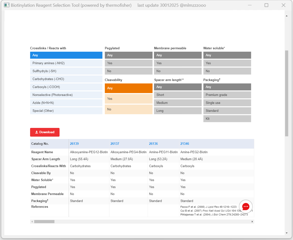
To identify new epitopes, specific experimental methods need to be designed to determine the surface frequency of each amino acid in AQP0 (i.e., to assess whether it is located on the protein surface and can specifically bind to ligands such as targeting peptides). Since different amino acids can specifically react with different biotinylation reagents in a quantifiable manner, the identification of suitable biotinylation reagents is critical to the success of the experiment. Based on this principle, we integrated the Biotinylation Reagent Selection Tool (BRST) (Fig.4) [5], which includes an open-source platform developed by Thermo Fisher, into the WebScrawler submodule of Matthew. This integration facilitates the rapid screening of potential biotin labeling reagents for wet-lab experiments, serving as the foundation for the subsequent BoolAcid submodule.
Fig. 4 | The page of the BRST (powered by ThermoFisher), an open-source platform, aids in selecting biotinylation reagents for wet-lab, mainly based on parameters such as spacer arm length, crosslinking reactivity, membrane permeability, and water solubility, to optimize experimental design for specific AA surface frequency determination.
Source Code (Code.4) has been uploaded on GitHub, and can be viewed below:
Code.4 | Source code of WebCrawler module
import sys
from PyQt5.QtCore import QUrl
from PyQt5.QtWidgets import QApplication, QMainWindow, QVBoxLayout, QWidget
from PyQt5.QtWebEngineWidgets import QWebEngineView, QWebEnginePage

print('''
^^ProEpiphary^^ ''')
print('''
Module: Matthew-WebCrawler 3.5''')
print('''
analyzing...''')
class WebApp(QMainWindow):
    def __init__(self):
        super().__init__()
        self.setWindowTitle("Biotinylation Reagent Selection Tool (powered by thermofisher)     last update 30012025 @mlmzzzooo")
        self.setGeometry(100, 100, 1200, 800)

        self.browser = QWebEngineView()
        self.browser.setUrl(QUrl("https://www.thermofisher.cn/cn/zh/home/life-science/protein-biology/protein-labeling-crosslinking/biotinylation/biotinylation-reagent-selection-tool.html"))

        self.browser.page().runJavaScript("""
            var unwantedElements = document.querySelectorAll('header, footer, .nav, .sidebar, .content-header, .other-unwanted-elements');
            unwantedElements.forEach(function(el) {
                el.style.display = 'none';
            });

            var tables = document.querySelectorAll('table');
            tables.forEach(function(table, index) {
                if (index == 0 || index == 1) {
                    table.style.display = 'block';
                } else {
                    table.style.display = 'none';
                }
            });

            var allElements = document.body.querySelectorAll('*');
            allElements.forEach(function(el) {
                if (el.tagName !== 'TABLE' && el !== tables[0] && el !== tables[1]) {
                    el.style.display = 'none';
                }
            });
        """)

        central_widget = QWidget()
        layout = QVBoxLayout()
        layout.addWidget(self.browser)

        central_widget.setLayout(layout)
        self.setCentralWidget(central_widget)

app = QApplication(sys.argv)
window = WebApp()
window.show()
sys.exit(app.exec_())
ii. BoolAcid
Before coding, it is crucial for us to firstly embody several mathematical modeling concepts, named as the Amino Acid to Bool Model (AABM), particularly related to sorting, quantification, and threshold determination.
1. Calculation of Solvent Accessible Surface Area (SASA) and Sorting
This sorting step is foundational of AABM for determining the exposure of amino acids to chemical reagents. Mathematically, this could be represented as:
L is the reordered list of amino acids based on their SASA values
2. Quantitative Chemical Modification and Frequency Measurement
Like the method we used in (Format.6), this step firstly focuses on quantifying the modification frequency θi.
The modification frequency θ can be seen as a proportion of the amino acid modification, which may depend on several experimental measurements (e.g., fluorescence, mass spectrometry [6]). The process repeats several times to obtain a mean modification frequency θ, which is used to define the Surface Exposure Rate (SER) γ of each amino acid. Also, this step involves averaging over multiple trials to reduce measurement variability:
On L, amino acids with SASA values (by calculation) in the top γ are classified as Boolean true (1), while those in the bottom (1-γ) are classified as Boolean false (0).
\[L_{\text{Bool}}(i) = \begin{cases}
1 & \text{if SASA}_i \text{ is in the top } \gamma \\
0 & \text{if SASA}_i \text{ is in the bottom } (1-\gamma)
\end{cases} \quad \color{gray}{\textit{(Format.11)}}\]
where SASAi is the SASA of the i-th amino acid in the sorted list L.
And after completing the above steps, we will obtain a reordered sequence, which is the core of the results of AABM, as shown in the table (Table.2) below (for illustration purposes only, not representative of any actual conditions):
Table.3 | An example of reordered sequence.
Position
Bool Value (By experiment)
SASA (Ų) (By computational calculation)
1
0
0.01
2
0
0.05
3
0
0.59
...
n-8
0
6.23
n-7
1
7.22
n-6
0
8.01
n-5
0
8.69
n-4
1
9.11
n-3
0
9.55
n-2
1
10.23
n-1
0
10.90
n
1
11.56
...
N-2
1
56.26
N-1
1
59.22
N
1
63.18
The mixed region is located between two ellipses.
4. Threshold Region Identification
The Boolean sequence LBool exhibits a transition from 0 to 1, with a mixed region in between (also shown in Table.2). This mixed region is identified as the threshold region LThreshold, which separates exposed and non-exposed amino acids. This region can be modeled as a range of indices where the value of LBool changes from 0 to 1.
5. Likelihood Threshold Determination
The final step of AABM is to determine the value of likelihood threshold. The threshold λ is determined by selecting a specific likelihood cutoff within the threshold region LThreshold. This likelihood cutoff corresponds to a specific SASA value, which defines the experimental threshold. Mathematically, this is expressed as:
where P(SASA|LThreshold) represents the likelihood function of SASA values within the threshold region.
6. Coding and results
Based on the aforementioned steps of AABM, we developed the AcidBool program, which implements the aforementioned principles and functions using Machine Learning methods. The source code has been uploaded on GitHub, some of the crucial part (for implementing the SASA reordered sequence) is shown below (Code.5).
Code.5 | Source code of SASA calculation module
#Only a portion of the core code is displayed. For the complete code, view GitHub.
#All paths in this code block are relative paths.

import nglview as nv
import freesasa
import os
import pandas as pd
from Bio import PDB
from IPython.display import display

def get_residue_names(pdb_file):
    parser = PDB.PDBParser(QUIET=True)
    structure = parser.get_structure("protein", pdb_file)
    residue_map = {}

    for model in structure:
        for chain in model:
            for residue in chain:
                if PDB.is_aa(residue, standard=True):
                    chain_id = chain.id.upper()
                    res_id = residue.get_id()
                    res_num = str(res_id[1])
                    if res_id[2] != " ":
                        res_num += res_id[2]
                    res_name = residue.get_resname()
                    residue_map[(chain_id, res_num)] = res_name

    return residue_map

def visualize_pdb(pdb_file):
    if not os.path.exists(pdb_file):
        print(f"error: PDB file '{pdb_file}' does not exist, check file path!")
        return None
    try:
        view = nv.show_file(pdb_file)
        display(view)
        return view
    except Exception as e:
        print(f"An error occurred while visualizing the PDB: {e}")
        return None

def calculate_sasa(pdb_file, output_xlsx="sasa_results.xlsx"):
    if not os.path.exists(pdb_file):
        print(f"error: PDB file '{pdb_file}' does not exist, check file path!")
        return

    try:
        structure = freesasa.Structure(pdb_file)
        result = freesasa.calc(structure)
        sasa_values = result.residueAreas()

        residue_names = get_residue_names(pdb_file)

        sasa_list = []

        for chain in sasa_values:
            for resnum, residue_area in sasa_values[chain].items():
                total_sasa = residue_area.total
                res_name = residue_names.get((chain.upper(), str(resnum)), "UNK")
                sasa_list.append([chain, resnum, res_name, total_sasa])

        df_sasa = pd.DataFrame(sasa_list, columns=["Chain", "R.No.", "Amino Acid", "SASA (Ų)"])
        df_sasa = df_sasa.sort_values(by="SASA (Ų)", ascending=True).reset_index(drop=True)

        df_sasa.to_excel(output_xlsx, index=False)
        print(f"\nSASA calculation completed, see result blank in: {output_xlsx}")

        print("\nSASA calculation result example (Sorted by SASA from smallest to largest):")
        display(df_sasa)

    except Exception as e:
        print(f"an unexcepted error occurred: {e}")

pdb_file = input("input PDB input-file path (or Enter with using '1ymg_chainA.pdb'):").strip()
if not pdb_file:
    pdb_file = r"1ymg_chainA.pdb"

output_xlsx = input("input Excel output-file path (or Enter with using 'sasa_results.xlsx'):").strip()
if not output_xlsx:
    output_xlsx = "sasa_results.xlsx"

view = visualize_pdb(pdb_file)
calculate_sasa(pdb_file, output_xlsx)
Table.4 | Samples of SASA reordered sequence of AQP0
Given that designing peptides targeting known sites on AQP0 may interfere with its normal physiological functions [7][8], and that peptide binding to AQP0 could trigger cellular pinocytosis [9], we firstly developed EpiFind in Elijah.
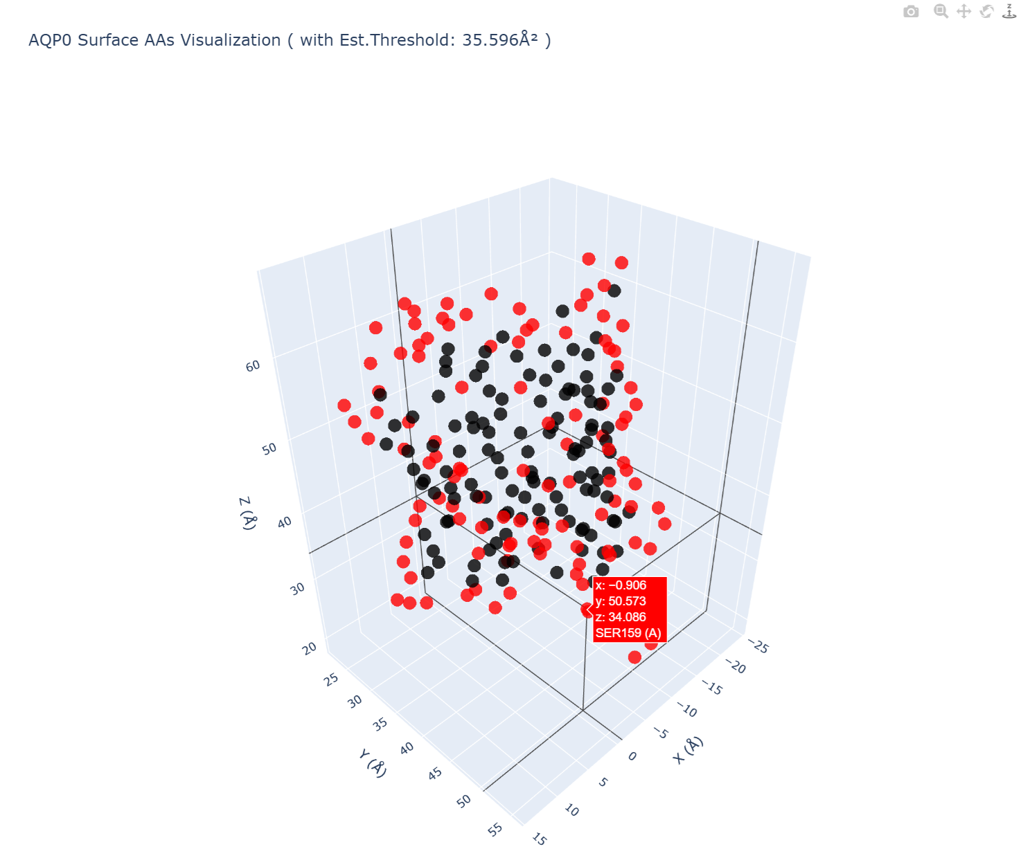
As a computational program for epitope identification and screening by integrating outputs from Matthew Module, EpiFind employs a Hierarchical Attention Network (HAN) to evaluate physicochemical environments and biological spatial conformational features through weighted feature analysis, which has been proved that are more efficient and accurate [10], thereby generating an initial set of potential novel epitopes on AQP0 (results shown below in Fig.5, source code in Code.6). These candidate epitopes are subsequently transferred to DeepPepGen for de-novo peptide generation.
Fig.5 | A screenshot of an interactive 3D visualization of AQP0 surface residues, highlighting solvent-accessible amino acids (those whose SASA > threshold, for whole data, click here to download the table) in red, with full rotation, zoom, and hover functionality for detailed structural analysis in following processes. For an interactive page (in HTML format), click here to open.
ii. DeepPepGen
Looking forward, DeepPepGen is positioned to serve as the final predictive module in targeted peptide design pipelines. With sufficient development time and wet-lab experimental data for model training in subsequent phases, its ultimate objectives may include:
Achieving end-to-end intelligent design of AQP0-binding peptides and providing direct candidate selections for drug conjugate components to experimental teams
Establishing a generalizable framework extendable to other protein-protein interaction prediction tasks
Code.6 | Source code of EpiFind module
#All paths in this code block are relative paths.

import pandas as pd
from biopandas.pdb import PandasPdb
import plotly.graph_objects as go
import numpy as np
import webbrowser

print('''^^ProEpiphary^^ ''')
print('''Module: Elijah-EpiFind 3.5''')
print('''analyzing...''')

sasa_df = pd.read_excel(r"C:\Users\11960\Documents\zju\sasa_results.xlsx")
non_zero_sasa = sasa_df[sasa_df["SASA (Ų)"] > 0]["SASA (Ų)"]
threshold = non_zero_sasa.median() if len(non_zero_sasa) > 0 else 0.0
threshold = 35.596   #Likelihood Threshold Replacement
print(f"Threshould: {threshold:.3f} Ų")

ppdb = PandasPdb().read_pdb(r"1ymg_chainA.pdb")
atom_df = ppdb.df['ATOM']

# Get CA atoms
ca_df = atom_df[atom_df['atom_name'] == 'CA'].copy()
ca_df['residue_number'] = ca_df['residue_number'].astype(int)

# Create SASA lookup dictionary
sasa_dict = {(row['Chain'], row['R.No.']): row['SASA (Ų)']
             for _, row in sasa_df.iterrows()}

# Color mapping based on SASA threshold
colors = []
surface_residues = []

for _, row in ca_df.iterrows():
    chain = row['chain_id']
    res_no = row['residue_number']
    res_name = row['residue_name']

    sasa = sasa_dict.get((chain, res_no), 0.0)

    if sasa > threshold:
        colors.append("red")
        surface_residues.append({
            "Chain": chain,
            "Residue Number": res_no,
            "Amino Acid": res_name,
            "SASA (Ų)": sasa
        })
    else:
        colors.append("black")

# Create 3D visualization
fig = go.Figure(data=[
    go.Scatter3d(
        x=ca_df['x_coord'],
        y=ca_df['y_coord'],
        z=ca_df['z_coord'],
        mode='markers',
        marker=dict(
            size=7.5,
            color=colors,
            opacity=0.8
        ),
        hovertext=[
            f"{row['residue_name']}{row['residue_number']} ({row['chain_id']})"
            for _, row in ca_df.iterrows()
        ]
    )
])

fig.update_layout(
    title=f"AQP0 Surface AAs Visualization ( with Est.Threshold: {threshold:.3f}Ų )",
    scene=dict(
        xaxis_title='X (Å)',
        yaxis_title='Y (Å)',
        zaxis_title='Z (Å)',
        aspectmode='data'
    ),
    width=1200,
    height=1000
)

fig.show()
fig.write_html(r"Surface_AAs_3D_View.html")
webbrowser.open("Surface_AAs_3D_View.html")

# Save surface residues to Excel
surface_df = pd.DataFrame(surface_residues)
surface_df = surface_df.sort_values(by=["Chain", "Residue Number"])

output_path = r"Surface_AAs.xlsx"
surface_df.to_excel(output_path, index=False)
print(f"Results already saved to: {output_path}")
In the future, we will continue to optimize the model and expand its application scope.
iii. DeepPepGen
At the beginning of WP, we planned to develop DeepPepGen as a whole-process affinity prediction platform that can automatically generate target peptide from the learning of AQP0. However, it is not a small feat. Due to the absence of established standard datasets and the practical challenges in obtaining direct wet-lab experimental validation data during WP phase, it remains particularly challenging to complete full-scale code implementation and model training for DeepPepGen at this stage. Considering these constraints, in WP, this section will primarily focus on:
Elaborating design rationale through comprehensive literature review and analysis of existing computational models
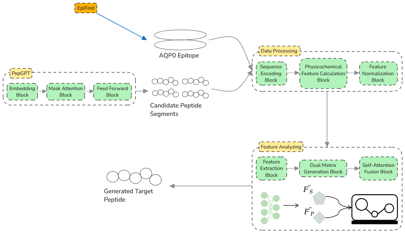
Presenting the conceptual framework architecture of DeepPepGen through schematic diagrams (Fig.6)
Fig.6 | Framework of DeepPepGen. Peptide segments are processed through PepGPT [11] for encoding, followed by feature extraction, physicochemical calculation, and normalization. The refined features are then combined using dual matrix generation [12] and Self-Attention Fusion (SAF) [13] blocks to generate the target peptide with high prediction score of affinity for wet-lab to advance Drug Conjugation process.
Looking forward, DeepPepGen is positioned to serve as the final predictive module in targeted peptide design pipelines. With sufficient development time and wet-lab experimental data for model training in subsequent phases, its ultimate objectives may include:
Achieving end-to-end intelligent design of AQP0-binding peptides and providing direct candidate selections for drug conjugate components to experimental teams
Establishing a generalizable framework extendable to other protein-protein interaction prediction tasks
Outlook: Let Eyes Behold the Light
"The light shineth in darkness; and the darkness comprehended it not. (John 1:5, KJV)" Every time, in those midnights when I toss and turn before the flickering screen, such verses lingered always crossed my mind and gave me strength, like dawnlight through the valley of the shadow (Psalm 23:4).
Life stands as our mutual magnum opus, and when the revelation of "Let there be light" (Genesis 1:3) is proclaimed, our lucent eyes became the most precious gift through which life allowed us to commune with all creation. I just always muse: to decode life's ciphers through inspired algorithms, letting truth's radiance dissolve the veils of obscurity, that all may freely behold "fields, woods, towns, rivers, clouds, sunshine, and all that lies before us" (Charlotte Brontë, Jane Eyre)—and I believe this just embodies the very essence that iGEM advocates, where neo-synthetic biology will embrace modeling, coding, software and AI to unveil the used-to-be hidden harmonies like protein design or drug discovery, expanding the frontier of human ingenuity indefatigably.
In all with zeal I hope, that our codes and methods may just translate into more healing visions, that through crystalline polypeptides we may weave light's lexicon, and sincerely, that no one left behind, we all, in our shared pilgrimage through science, may truly become the light of the world (Matthew 5:14).
References
[1]Yoon, B. J. (2009). Hidden Markov Models and their Applications in Biological Sequence Analysis. Current genomics, 10(6), 402–415.DOI: 10.2174/138920209789177575
[2]Li, J., Lee, JY., & Liao, L. (2021). A new algorithm to train hidden Markov models for biological sequences with partial labels. BMC Bioinformatics, 22, 162.DOI: 10.1186/s12859-021-04080-0
[3]Porter, T. M., Hajibabaei, M. (2021). Profile hidden Markov model sequence analysis can help remove putative pseudogenes from DNA barcoding and metabarcoding datasets. BMC Bioinformatics, 22, 256.DOI: 10.1186/s12859-021-04180-x
[4]Delgado-Bonal, A., & Marshak, A. (2019). Approximate Entropy and Sample Entropy: A Comprehensive Tutorial. Entropy, 21(6), 541.DOI: 10.3390/e21060541
[5]Thermo Fisher Scientific. (n.d.). Biotinylation reagent selection tool. Thermo Fisher Scientific. Retrieved February 2, 2025, from thermofisher.com
[6]Spickett, C. M., & Pitt, A. R. (2012). Protein oxidation: role in signalling and detection by mass spectrometry. Amino acids, 42(1), 5-21.DOI: 10.1007/s00726-010-0585-4
[7]Schey, K. L., Wang, Z., Wenke, J., & Qi, Y. (2014). Aquaporins in the eye: expression, function, and roles in ocular disease. Biochimica et biophysica acta, 1840(5), 1513–1523.DOI: 10.1016/j.bbagen.2013.10.037
[8]Gutierrez, D. B., Garland, D. L., Schwacke, J. H., Hachey, D. L., & Schey, K. L. (2016). Spatial distributions of phosphorylated membrane proteins aquaporin 0 and MP20 across young and aged human lenses. Experimental eye research, 149, 59–65.DOI: 10.1016/j.exer.2016.06.015
[9]Wang, Z., & Schey, K. L. (2011). Aquaporin-0 interacts with the FERM domain of ezrin/radixin/moesin proteins in the ocular lens. Investigative ophthalmology & visual science, 52(8), 5079-5087.DOI: 10.1167/iovs.10-6998
[10]Mousavi, S., Afghah, F., Acharya, U. R. (2020). HAN-ECG: An interpretable atrial fibrillation detection model using hierarchical attention networks. Computers in Biology and Medicine, 127, 104057.DOI: 10.1016/j.compbiomed.2020.104057
[11]Rehana, H., Çam, N. B., Basmaci, M., Zheng, J., Jemiyo, C., He, Y., Özgür, A., & Hur, J. (2023). Evaluation of GPT and BERT-based models on identifying protein-protein interactions in biomedical text. ArXiv, arXiv:2303.17728v2.
[12]Yang, M., et al. (2023). MIX-TPI: A flexible prediction framework for TCR-pMHC interactions based on multimodal representations. Bioinformatics, 39(8), btad475.DOI: 10.1093/bioinformatics/btad475
[13]Shin, B., Park, S., Kang, K., & Ho, J.C. (2019). Self-Attention Based Molecule Representation for Predicting Drug-Target Interaction. Proceedings of the 4th Machine Learning for Healthcare Conference, 106:230-248.Link to paper